The Versatile Asset:
Portfolio Construction with Private Credit

White Paper

Read Time: 18 minutes

You Will Learn:

Private credit, particularly direct lending, offers diversification benefits to traditional 60/40 portfolios.
Direct lending has historically generated high and consistent income returns, which can boost the overall portfolio yield, providing stable cash flows and mitigating volatility from other portfolio components.
Private credit allocation strategies may help investors achieve specific goals, such as enhancing retirement income, increasing endpoint wealth or replacing traditional credit exposures.

Diversified and Diversifying

An Untapped Opportunity for Portfolio Resilience

This analysis takes as its “base case” a typical generic portfolio of equities (60% via the S&P 500) and bonds (40%, proxied by the Bloomberg U.S. Aggregate). While it’s very much of the moment to impugn the traditional 60/40 portfolio, it remains a longstanding and reasonable starting point or home base.

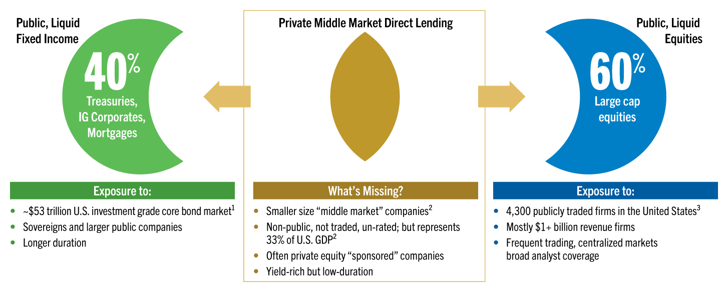
Moreover, regardless of the specific starting portfolio, it’s no stretch to argue that the vast majority of most allocations today over-weight large, publicly traded, liquid assets, mostly across investment grade firms or sovereigns with broad analyst or ratings agency coverage—whether on the debt or equity side of the portfolio (See Exhibit 1).

The simplest act of diversification is to incorporate in the portfolio “what’s different” or “what’s missing” from this usual mix of assets. Investors could find that missing link in smaller, private, less liquid and individually originated debt in unrated “middle market” companies that are often the target of investment by private equity sponsors.

These characteristics represent a clear and compelling complement or “yin” to the “yang” of the typical exposures in a 60/40 portfolio. But the dissimilarities to a generic investor portfolio continue, particularly on the bond side.

Where public debt is mostly fixed, directly originated loans are floating; where traditional fixed income is vulnerable to rate volatility and the erosion that inflation brings, direct lending has near-zero¹ duration risk and tends to rise along with the Consumer Price Index (“CPI”).

While most traditional bond holdings generated an anemic yield or income return over the last two decades, the returns from direct lending brought in double-digit levels of annualized income.²

Exhibit 1

The Missing Link: The Yin to a Portfolio’s Yang

Private Direct Lending Provides a Key Diversification Opportunity

1. Bloomberg U.S. Aggregate Bond Index. As of June 2024.
2. The National Center for the Middle Market defines the U.S. middle market as companies with annual revenues between $10 million and $1 billion, “Mid-Year 2024 Middle Market Indicator.” As of June 30, 2024.
3. CNN Business, “The stock market is shrinking and Jamie Dimon is worried.” As of April 9, 2024

Exhibit 2 represents a tally of some commonly referenced characteristics of direct lending. Some investors may be familiar with them individually, but it’s their combination that renders the asset class especially versatile and makes it a particularly effective portfolio diversifier.

Arguably the most appealing performance characteristic for clients and advisors is the double-digit annualized income generated over the last 20 years by the asset class. DL has provided consistent cash flows for client spending and has helped to stabilize the natural periodic volatility coming from other areas of the portfolio.

While income is the bedrock, direct lending’s total returns include a “capital appreciation” component driven by realized credit gains or losses. As can be deduced from the numbers, over 20 years, that has averaged to an annual credit loss rate of just over 1%, haircutting yearly total returns to just under 10%.

From a risk perspective, this illiquid asset consists of bespoke, private loans that have no public market and are typically valued on a monthly or quarterly basis. Since there is little contagion from centralized public market volatility, direct lending returns tend to move more slowly than their public counterparts—they have generally low standard deviation or volatility.³

The loans are also senior in the capital stack, secured by cash flows and collateral, first to be paid out and the last to lose value in the event of default. They are floating rate, valued at a consistent spread to SOFR, and have near-zero duration: Rising fed fund rates buoy the “base rate” upon which the loans are priced; in falling rate periods, they fare well, benefitting from lower debt-funding costs and improved credit dynamics across their portfolio companies.

In part due to their floating rate character, but also thanks to the nature of the companies in the portfolio (essentially non-public small cap equities), direct lending returns tend to rise with CPI and thus may provide inflation-mitigation to an otherwise vulnerable bond portfolio. And relative to the traditional fixed income allocation, direct lending tends to have a very low or, in some cases, negative correlation, which can bring greater diversification benefits and superior efficiency to the portfolio’s overall risk and return profile.

Exhibit 2

A Rare Combination of Virtues

Direct lending possesses a rare combination of characteristics otherwise in low supply among traditional portfolio components.

High and consistent yield
10.9% annualized¹; income-enhancing

High total returns
9.5% annualized¹; may buoy growth

Low volatility
3.5% over 20 years¹; may reduce portfolio standard deviation

Senior in the capital stack
For capital preservation; reduces credit risk

Almost zero duration
May reduce interest rate risk in the portfolio

Strong correlation with CPI
May reduce portfolio vulnerability to rising inflation

Low correlations to the rest of the portfolio
Negative correlation to traditional bonds; could improve Sharpe Ratio

1. Cliffwater Direct Lending Index (“CDLI”). As of June 30, 2024.

For a Portfolio-Enhancing Income Boost

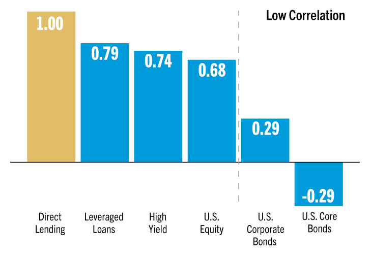
One key element that renders any new asset of interest is its relationship to the rest of the portfolio, and in particular its differences: how it combines and behaves with other assets. The left side of Exhibit 3 illustrates direct lending’s correlation to its public sub-investment grade peers (leveraged loans and high yield) and to equities broadly, as well as traditional fixed income.

While there is a natural similarity of behavior across the three sub-investment grade siblings, the correlation drops precipitously when we move to the right, to corporate credit and its broader “core” proxy, the U.S. Aggregate index, typically the largest allocation in most clients’ bond portfolios.

This may prompt early thinking about sourcing—where to create space in the portfolio (from similar-behaving assets) and the benefits of blending the new allocation (with low-correlation to the rest) into the total portfolio.

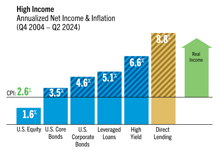
Meanwhile, the right side of Exhibit 3 isolates direct lending’s “super power” characteristic—its income return, suggesting its value as a driver of “real” income or yield beyond the level of inflation. Combine these two attributes, and direct lending may be seen, at its essence, as providing a portfolio-diversifying income boost.

Exhibit 3

Low Correlation and High Income

Direct Lending Offers a Portfolio-Diversifying Income Boost

Direct lending is an intuitive replacement for other credit and equity exposures and blends well (due to low correlations) with traditional fixed income components.

With its historically high and consistent net income, direct lending in almost all cases will help boost overall portfolio “real” yield when included in a strategic allocation.

Note: Direct Lending is represented by the CDLI; High Yield is represented by the ICE BofA U.S. High Yield Index. The ICE BofA U.S. High Yield Index tracks the performance of dollar-denominated, below-investment-grade corporate debt publicly issued in the U.S. domestic market. Leveraged Loans are represented by the Morningstar LSTA U.S. Leveraged Loan Index. The Morningstar LSTA U.S. Leveraged Loan Index is a market value–weighted index designed to measure the performance of the U.S. broadly syndicated leveraged loan market. The Morningstar LSTA U.S. Leveraged Loan Index typically encompasses 90%–95% of the entire broadly syndicated leveraged loan market. U.S. Corporate Bonds are represented by the Bloomberg U.S. Corporate Index. U.S. Core Bonds are represented by the Bloomberg U.S. Aggregate Bond Index. The Bloomberg U.S. Aggregate Bond Index represents securities that are SEC registered, taxable and dollar denominated. The index covers the U.S. investment-grade fixed-rate bond market, with index components for government and corporate securities, mortgage pass-through securities and asset-backed securities. These major sectors are subdivided into more specific indices that are calculated and reported on a regular basis. U.S. Equity is represented by the S&P 500 index, a market capitalization– weighted index of 500 leading publicly traded companies. Note: Past performance does not guarantee future results. You cannot invest directly in an index, which also does not take into account trading commissions and costs. The volatility of indices may be materially different from the performance of Golub Capital Funds. Index returns reflect all items of income, gain and loss and the reinvestment of dividends and other income. September 30, 2004–June 30, 2024. Correlation is a statistical measure of the degree to which the prices of two securities move in relation to each other. A correlation of 1 means the prices always move in the same direction. A correlation of −1 means the prices always move in opposite directions. The correlation calculation is based on quarterly net returns. This page is accompanied by the Important Investor Information at the end of this document, which is an integral part of this presentation. Gross income is reduced by estimated fund-level fees and expenses as measured by CDLI and The Investment Company Institute 2024 Factbook for representative asset classes. See the Appendix for the fee analysis and for both gross and net returns details. Time period analyzed Q4 2004 (since CDLI inception) to Q2 2024, returns and volatilities presented on an annualized basis.

Optimizing the Income Efficient Frontier

The next analysis focuses further on the income theme as the most distinctive attribute of the asset class. Exhibit 4 borrows the concept and layout of a traditional efficient frontier, with volatility or standard deviation on the x-axis.

But instead of using total return as the metric for the y-axis, the analysis substitutes income return. The blue line, starting on the far right, shows the 20-year annualized volatility of equities (at about 16%) and the income return from dividends at approximately 1.5% annualized.⁴

Tracking the blue line left to the 100% bond portfolio (using here the U.S. Aggregate for this traditional exposure), it shows a volatility of 4%, along with an annualized coupon income of just over 3%. The full visual represents an “income- oriented efficient frontier.”

The “base case” 60/40 allocation occupies the center, with about 10% annualized volatility and with a 2.3% “income return” over the last 20 years. The gold line moving up and left reflects a gradually increasing substitution of direct lending into the 60/40 allocation, at increments of 10% up to 40% exposure.⁵

An allocation of that amount is clearly outsized in nature but useful for illustrative purposes: The allocation with 20% in DL generates 56% higher income return, while the 40% allocation delivers a 112% increase in portfolio income over the last 20 years.

The line reflecting the incrementally larger DL allocation tilts to the left, indicating a simultaneous decrease in volatility, in part driven by the alchemy of the asset’s low correlation to both bonds and equities but also by its lower volatility (lower than equities). The dramatic north-west tilt in the gold line shows the diversifying income-impact of incorporating DL in the portfolio. This illustration helps isolate further the potent income return of direct lending and underlines its appeal to individual investors.

Exhibit 4

Recalibrating the Efficient Frontier: From Total Return to Income

(Optimizing for Income with Direct Lending)

Note: Equities returns are represented by the S&P 500, Bonds by Bloomberg U.S. Agg. DLs are represented by the unlevered CDLI index. Net NAV DL income and total return are reduced by estimated fund-level fees and expenses totaling 193 bps. Equities income/total return are reduced by estimated fees = 42 bps, Bonds by 37 bps. Allocation to DL is sourced 65% from equity and 35% from bonds, i.e., portfolio with 10% DL allocation is 57% stocks and 33% bonds. Time period analyzed Q4 2004 (since CDLI inception) to Q2 2024, returns and volatilities presented on annualized basis. See the Appendix for fees and gross and net returns details. Suggested allocations will vary depending on constraints applied; recommended sourcing is derived from many factors, including relative correlations, volatilities, returns and income for each asset alone and in combination with the other two.

Allocation Alchemy: Sourcing

Optimal Sourcing for the Direct Lending Allocation

Most institutional allocation studies do not bother much with the question of how a new exposure is “sourced”— how to make room for the new asset by selling existing assets. Advisors know this is not a trivial exercise but requires thorough analysis: It’s not just “how much” of the new asset to import into the portfolio; the question “from where” is critical and often underappreciated.

Exhibit 5 illustrates the calculus involved—how different approaches to sourcing the new exposure involve multiple trade-offs that an advisor must navigate. And all of these trade-offs tie back to the client’s goals and desired outcome, the advisory north star in all of this.

Beginning with the base case of 60/40 and embedding the 20-year risk-and-return history and associated fees of all three asset categories, the analysis looks across four key dimensions of portfolio performance: Income Return, Total Return, Volatility and Sharpe Ratio (a measure of portfolio utility or efficiency).

The analysis illustrates two extreme positions on either end to show in stark relief some of the trade-offs: sourcing the DL allocation either 100% from bonds or 100% from equities. The results are intuitive to some: Pulling entirely from equities, which tend to have much lower income return and higher volatility than direct lending, will result in the highest improvement in those areas, increasing the income return by over 60% and reducing standard deviation by 27%—while modestly reducing the total return (by −7%).

Conversely, pulling entirely from bonds, which already have low volatility and lower total returns but are income-producing by nature, will result in a more modest improvement in income return (+47%) relative to the equity-sourced example but a larger improvement (+12%) in total return (and just a bit higher volatility). In both cases, portfolio efficiency is improved, but thanks to the much lower volatility when sourcing from equities, the impact is greater there. With this sourcing framework in mind, the advisor can bring more precision to the effort of fine-tuning the new allocation to meet a client’s distinct investment goals.

Exhibit 5

Measuring the Trade-Offs: Sourcing from Equities or Bonds

(Results Based on a 20% Direct Lending Allocation)

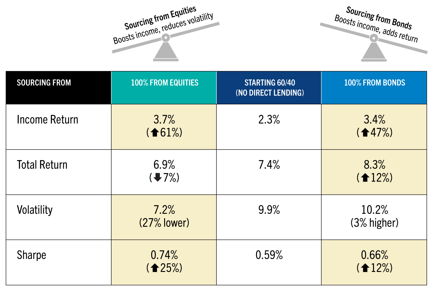
Note: Equities and bond returns are represented by the S&P 500 and Bloomberg U.S. Agg respectively. DLs are represented by the unlevered CDLI index. Net NAV DL income and total return are reduced by estimated fund-level fees and expenses totaling 193 bps. Stock and bond income/total return are reduced by estimated fees = 42 bps and 37 bps respectively. Time period analyzed Q4 2004 (since CDLI inception) to Q2 2024, returns and volatilities presented on an annualized basis. See the Appendix for fees and gross and net returns details. Suggested allocations will vary depending on the constraints applied; recommended sourcing is derived from many factors, including relative correlations, volatilities, returns and income for each asset alone and in combination with the other two.

Client Goal #1:
Retirement Income

Meet Annual Spending Target

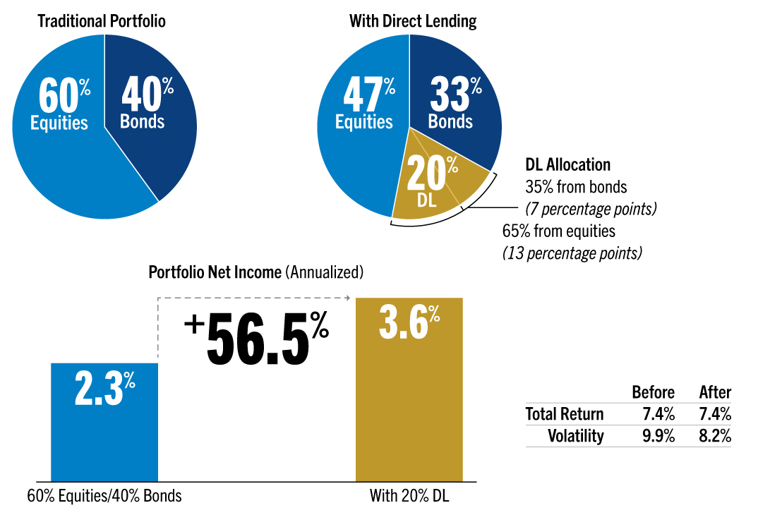
Consider the client whose primary goal is to enhance the income return or cash flows their portfolio throws off, but without seeing any appreciable drop in total return. If there are ancillary benefits, in terms of volatility reduction or a higher Sharpe Ratio, she’ll accept those as well.

From a starting 60/40 portfolio and base case allocation of 20% in direct lending, the goal is to optimize for the highest income return while holding the original 60/40 portfolio’s total returns steady at 7.4%.

With this goal in mind, an optimal sourcing strategy would pull the majority of the DL allocation (65% of it, or 13 percentage points of the total 20%) from equities and the remainder of the 20% allocation (7 percentage points) from bonds (see Exhibit 6).

This results in more than a 50% improvement in income return to 3.6% annually versus the base case of 2.3%.

Total returns hold steady at 7.4%, and there’s an additional benefit of reduced volatility (9.9% to 8.2%). This exercise illustrates in general terms a thoughtful advisory approach to optimize for a distinct and rather common client goal.

The next step is to apply this type of analysis to an actual client situation.

Exhibit 6

A Versatile Asset: Optimizing the Client Allocation to Enhance Income

For the investor seeking to maximize income return while keeping the same level of total return

Note: Equities and bond returns are represented by the S&P 500 and Bloomberg U.S. Agg respectively. DLs are represented by the unlevered CDLI index. Net NAV DL income and total return are reduced by estimated fund-level fees and expenses totaling 193 bps. Stock and bond income/total return are reduced by estimated fees = 42 bps and 37 bps respectively. Time period analyzed Q4 2004 (since CDLI inception) to Q2 2024, returns and volatilities presented on an annualized basis. See the Appendix for fees and gross and net returns details. Suggested allocations will vary depending on constraints applied; recommended sourcing is derived from many factors, including relative correlations, volatilities, returns and income for each asset alone and in combination with the other two.

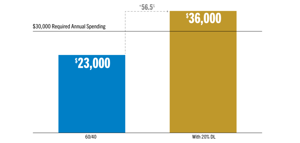
The investment goal of enhancing portfolio income does not exist in a vacuum. Clients think in real, applied terms, and advisors need to help them understand and pre- experience the value generated through thoughtful asset allocation. Exhibit 7 shows how this generic goal aligns with a fairly typical client situation—retirement portfolio construction and specifically “decumulation” or the need to deliver cash flows to support retiree spending.

In this example, a 65-year-old retiree has a $1 million portfolio allocated 60/40, which generates 2.3% or $23,000 per annum in income. The client is already taking Social Security in the amount of $30,000 each year. But her annual spending is closer to $60,000 a year.

So she’s seeking to generate at least $30,000 from her asset portfolio to reach that income target, and so far she’s not. Incorporating a 20% DL allocation, optimized for income (by sourcing it 65% and 35% from equities and bonds respectively), the new portfolio delivers over 50% improvement in annual income, to $36,000 per year. That’s more than enough to reach her spending target, with no loss in expected total returns (and with lower overall volatility).

Exhibit 7

Allocation in Action: The Retiree Solving an Annual Income Goal

A retiree with a 3% annual spending target, seeking to generate $30,000 per annum from her financial portfolio (with no loss in expected returns)

Seeking to Maximize Income Return Without Damaging Total Returns

For illustrative purposes only.

Note: Equities returns are represented by the S&P 500, Bonds by Bloomberg U.S. Agg. DLs are represented by the unlevered CDLI index. Net NAV DL income and total return are reduced by estimated fund-level fees and expenses totaling 193 bps. Equities income/total return are reduced by estimated fees = 42 bps, Bonds by 37 bps. Allocation to DL for retiree is sourced 65% from equity and 35% from bonds. Time period analyzed Q4 2004 (since CDLI inception) to Q2 2024, returns and volatilities presented on an annualized basis. See the Appendix for fees and gross and net returns details. Suggested allocations will vary depending on constraints applied; recommended sourcing is derived from many factors, including relative correlations, volatilities, returns and income for each asset alone and in combination with the other two.

Client Goal #2:
Maximize Endpoint Wealth

Seeking the Highest Wealth Outcome

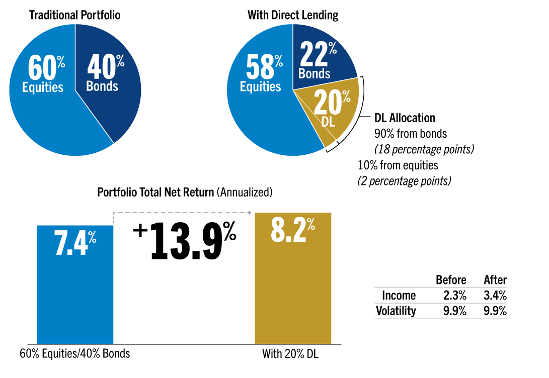
But there are different types of clients, with different goals. Take a younger professional, an “accumulator,” seeking to achieve greater total returns over time but without increasing portfolio volatility. We take our same 60/40 starting portfolio and our proposed 20% DL allocation, but in this case, to optimize for total returns, we now source the allocation almost entirely (90%) from the bond side of the portfolio.

So, 18 percentage points of the DL allocation will be sourced from traditional core bonds, and the remaining 2 percentage points will come from equities.
The results are shown in Exhibit 8.

Focus first on the improvement in total return, from the base case of 7.4% moving up to 8.2%, over 20 years— an improvement of nearly 14%. Portfolio volatility suffers no change, but the client also receives a nearly 50% improvement in income returns, from 2.3% to 3.4%.

These results may be more impactful when seen in the context of an actual client situation.

Exhibit 8

A Versatile Asset: Optimizing an Allocation to Enhance Total Returns

For the investor seeking to maximize total return without changing the overall volatility of the portfolio

Note: Equities and bond returns are represented by the S&P 500 and Bloomberg U.S. Agg respectively. DLs are represented by the unlevered CDLI index. Net NAV DL income and total return are reduced by estimated fund-level fees and expenses totaling 193 bps. Stock and bond income/total return are reduced by estimated fees = 42 bps and 37 bps respectively. Time period analyzed Q4 2004 (since CDLI inception) to Q2 2024, returns and volatilities presented on an annualized basis. See the Appendix for fees and gross and net returns details. Suggested allocations will vary depending on constraints applied; recommended sourcing is derived from many factors, including relative correlations, volatilities, returns and income for each asset alone and in combination with the other two.

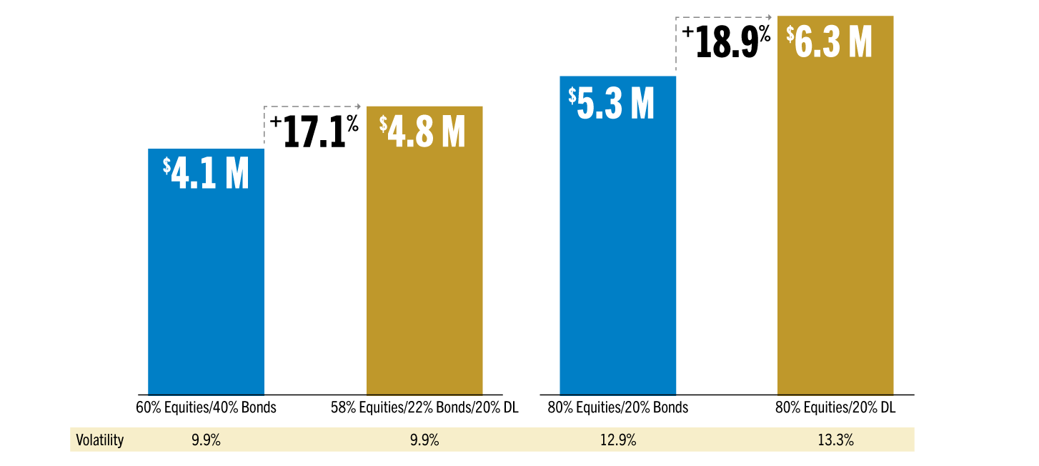
Take a younger, 45-year-old client, mid-career and spending from his paycheck with a long horizon portfolio. He’s looking to create the largest retirement nest egg possible. His focus is on higher returns and accelerated compounding (perhaps the assets are held in an IRA to limit tax headwinds), all to maximize long-term wealth.

Start with the 60/40 portfolio with $1 million in assets, running for 20 years without withdrawals: after 20 years, it generates $4.1 million in wealth (See Exhibit 9). If instead the client had diversified the portfolio with 20% in DL, in an allocation optimized to favor total return (sourcing the DL allocation 90% from bonds and 10% from equities), he’d instead have $4.8 million 20 years hence, at age 65: an increase of about 17% in final wealth—with essentially no change in volatility.

Now, if the client is comfortable with higher volatility and is willing to move to an 80% equity portfolio, given the long holding period, there is another option to consider.

The 80/20 equity/bonds allocation would rise from $1 million to $5.3 million over 20 years. But if he diversified with private credit, replacing the entire remaining bond portfolio (20% in the Agg) with direct lending, the final wealth outcome is $6.3 million, almost 20% higher.

This new allocation will carry slightly more volatility, with a standard deviation of about 13%. This is due to the higher equity allocation and from sourcing the DL allocation entirely from the remaining core bond portfolio. But that’s a compromise he was willing to make given the long-term horizon for this allocation.

These examples represent nuanced advisory conversations focused on optimizing the DL allocation within the total portfolio for very specific client goals—enhancing income and higher total return. But some situations may be far easier to address and require less subtlety.

Exhibit 9

Allocation in Action: Accumulator Seeks Highest Wealth Outcome

A younger professional seeking strong compounding and maximum wealth outcome over 20 years

$1 Million Invested in Q3 2004, After 20 Years, Net of Fees

Note: Equities returns are represented by the S&P 500, Bonds by Bloomberg U.S. Agg. DLs are represented by the unlevered CDLI index. Net NAV DL income and total return are reduced by estimated fund-level fees and expenses totaling 193 bps. Equities income/total return are reduced by estimated fees = 42 bps, Bonds by 37 bps. Allocation to DL for accumulator is sourced 90% from bonds and 10% from equities. Allocation to DL for accumulator with 80% equity allocation is sourced 100% from bonds. Time period analyzed Q4 2004 (since CDLI inception) to Q2 2024, returns and volatilities presented on an annualized basis. See the Appendix for fees and gross and net returns details. Suggested allocations will vary depending on constraints applied; recommended sourcing is derived from many factors, including relative correlations, volatilities, returns and income for each asset alone and in combination with the other two.

Client Goal #3:
Credit Replacement

A Credit-Replacement Approach

For clients who simply want to find a more efficient substitute for their current exposure to corporate credit, direct lending may be a solution. In this case, the client is simply looking at a one-for-one swap of their corporate credit allocation. Their current credit exposure may be a dedicated allocation to investment-grade corporate bonds, high-yield, or senior loans. And since this is a simple exchange of one exposure for the other, this renders the “sourcing” discussion moot.

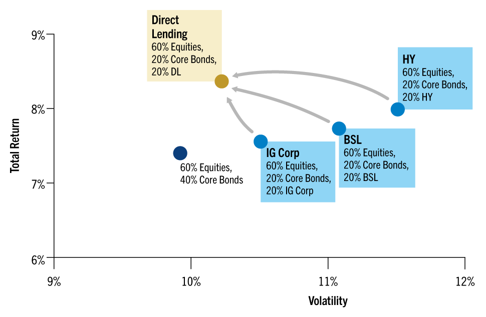
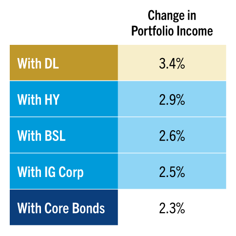
First, for context, the analysis situates the familiar starting allocation of 60% equities and 40% bonds, signified by the dark blue dot, with a total return of 7.4% and a volatility of 9.9% (See Exhibit 10). In the other “credit-oriented” bond allocations, the exposure is split between traditional core bonds (with 20% remaining in the U.S. Agg) and a more dedicated corporate credit exposure: 20% in either investment grade corporate bonds (IG Corp), high yield (HY) or leveraged loans (BSL) (shown by the three lighter blue dots).

The analysis swaps out each of the three public credit allocations (Corporate Credit, HY and Loans) for 20% in direct lending exposure. Looking over the 20-year return history of these assets, fees included, each outcome shows an improvement across the full portfolio in total return (on the Y axis), reduced volatility (on the X axis) and in the level of income thrown off by the portfolio (in the table to the right).

For HY, the improvement is most evident in a reduction in volatility; for Corporate Credit, the benefit is seen mostly around total returns. And the overall appeal of making the swap is amplified when you look at the higher portfolio income: as you move from from the bottom to the top of the accompanying table. From the “starting portfolio” of 2.3% (Agg-only) up to 2.5% with the 20% in IG Corporates, to 2.6% with 20% in senior loans, 2.9% with HY, and 3.4% with that 20% in DL. So, “credit replacement” turns out to be a rather simple case when it comes to direct lending.

Exhibit 10

A Superior Credit Allocation

(Improvement In Returns, Risk and Income)

Note: Equities returns are represented by the S&P 500, Core bonds, IG and HY by Bloomberg U.S. Agg, Bloomberg U.S. IG and Bloomberg U.S. HY respectively. Leveraged loans are represented by Morningstar LSTA. DLs are represented by the unlevered CDLI index. Net NAV DL income and total return are reduced by estimated fund-level fees and expenses totaling 193 bps. Stock income/ total return are reduced by estimated fees = 42 bps, Agg by 37 bps, IG by 27 bps, HY by 63 bps, Loans by 65 bps. Time period analyzed Q4 2004 (since CDLI inception) to Q2 2024, returns and volatilities presented on an annualized basis. See the Appendix for fees and gross and net returns details. Suggested allocations will vary depending on constraints applied; recommended sourcing is derived from many factors, including relative correlations, volatilities, returns and income for each asset alone and in combination with the other two.

Allocating for the Future

Now it’s time to adjust the lens in the analysis, moving from the full 20-year lookback, to turn instead to the next 20 years. No one has a crystal ball, of course, when considering future asset-class returns. But that shouldn’t stop advisors from at least laying out the question. As much of this analysis is based on historic risk-and-return data, it seems worth considering what many forecasters think may come in the future.

Looking at the past, investors have been afforded outstanding returns in equities, north of 10% (and this even after fees). And while bonds have provided far more modest returns during recent history (2.6% after fees), the much- maligned 60/40 portfolio has earned a respectable 7.4% net of fees. Had they allocated 20% of that 60/40 to DL in a sourcing optimized for total return (90% from bonds), they’d have seen 8.2% returns annualized for the 20-year period.

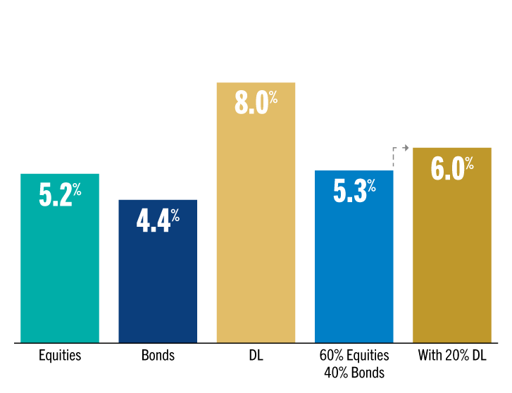
But turning to the next 20 years, a representative forecast suggests a far different future: one where equities deliver only half (5.2%) of what they had previously and where bonds return just a shade behind equities (at 4.5%). That leaves the traditional 60/40 portfolio with a mere 5.3% in expected net of fee returns. In this case, incorporating direct lending may be less of a “nice to have” and more of a necessity. Doing so would at least give the total future portfolio a 6% projected total return.

Regardless of the accuracy of these projections (which happen to agree with many similar forecasts available from the world’s most trusted firms), it’s important to consider any number of possible futures and to see where private credit might lend a hand.

Exhibit 11

Allocating for the Future: Direct Lending May Help Overcome Future 60/40 Headwinds

A Backward Glance
(Historical Annualized Net Returns)

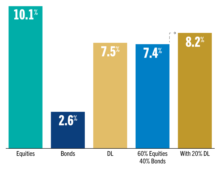
A Different Future
(Forecasted Annualized Net Returns)

Note: Modeling assumptions by Altar Rock LLC, initial market conditions as of September 1, 2024. Equities model based on U.S. Large Cap, Forward-looking Agg bonds allocation modeled as 50% 7yr Treasuries and 50% IG Credit, DL is based on CDLI. DL allocation is sourced 10% from equites and 90% from bonds. These illustrations should not be viewed as representative of other asset classes, mixes thereof or actual investment portfolios that may employ strategies not depicted here. Net NAV DL income and total return are reduced by estimated fund-level fees and expenses totaling 193 bps. Equities income/total return are reduced by estimated fees = 42 bps, Bonds by 37 bps. Forward-looking simulations are produced by proprietary research. While these are developed with care, there can be no guarantee of depicting the full range of potential future returns or of matching the true, unknown probabilities of outcomes.

The Right Asset in the Right Vehicle

As the discussion turns from historic analysis to an actionable future, it seems only right to take the next step and offer some perspective on the various pathways to investment in terms of vehicle options. There are three common approaches to obtaining exposure to the private direct lending space, ranging from publicly traded BDCs with daily liquidity to traditional “drawdown” LP funds with no interim liquidity and qualified purchaser requirements (exclusively for clients with a net worth of $5 million or more).

The publicly traded BDC is especially attractive for its instantaneity: it has no investor qualifications, no minimum investments and attractive 1099 tax treatment, among its virtues. But it also comes with a volatility that easily exceeds that of equities.

The private fund may be the “purest” form of exposure to these less liquid assets, but the restrictions on ownership, high minimums, absence of liquidity and onerous K-1 tax treatment may oblige most investors to look for another way.

The middle way, so to speak, is the non-traded BDC, which offers some of the benefits of both extremes: 1099 tax treatment, low minimums, lower “qualifications” to invest, a degree of liquidity (20% per annum, 5% quarterly) and more modest volatility than publicly traded BDCs. It may represent a happy medium for many.

This semi-liquid format provides what many today refer to as “democratized” access to this alternative investment; it retains the quality of true private market investing but delivers the exposure without some of the onerous tax and liquidity characteristics of long-duration drawdown funds.

Exhibit 12

Pros and Cons: The Right Asset in the Right Vehicle

Listed BDC

Public BDCs are listed on exchanges and offer immediacy of investment but much higher price volatility

Daily liquidity
Equity-like volatility
1099 tax treatment
Low minimums; traded online

Non-Traded BDC

Semi-liquid BDCs enable monthly
subscription at NAV and immediate allocation of proceeds

Monthly subs; quarterly redemption
Monthly NAVs; lower volatility
1099 tax treatment
Low minimum; subscription doc

Private Credit Fund

True “patient capital” funds, limited
to qualified purchasers, with assets
“called” over time and no interim
liquidity feature

No interim liquidity
Quarterly marks; lower volatility
K-1 tax treatment
High minimum; GP-LP agreements

Source: Golub Capital

1. Direct Lending is represented by the Cliffwater Direct Lending Index (“CDLI”). CPI is represented by the U.S. CPI Urban Consumers SA Index (“CDI”). Based on the correlation of CDLI’s quarterly returns and the quarterly change in CPI from September 30, 2004 through September 30, 2024.
2. Cliffwater Direct Lending Index (“CDLI”). As of June 30, 2024.
3. Returns are measured by annualized returns, which are calculated based on quarterly returns. Annualized volatility is measured by standard deviation of quarterly returns. Data from September 30, 2004 through December 31, Direct Lending is represented by the CDLI.
4. All the analyses in this paper (except for the forward-looking projection) reflect a 20-year history for each asset in the portfolio, rebalanced annually, and apply an average weighted fund fee to all of the assets in the study (average weighted fees are drawn from the Investment Company Institute 2024 Factbook or from Cliffwater research in the case of direct lending). See Endnotes for further
5. Sourcing for this “income efficient frontier” follows the approach described in Exhibit 5, indicating a blend of sourcing 65% of the DL exposure from equities and 35% from bonds, with the goal of maximizing income with no loss in return.

Disclaimer

In this document, the terms “Golub Capital” and “Firm” (and, in responses to questions that ask about the management company, general partner or variants thereof, the terms “Management Company” and “General Partner”) refer, collectively, to the activities and operations of Golub Capital LLC, GC Advisors LLC (“GC Advisors”), GC OPAL Advisors LLC (“GC OPAL Advisors”) and their respective affiliates or associated investment funds. A number of investment advisers, such as GC Investment Management LLC (“GC Investment Management”), Golub Capital Liquid Credit Advisors, LLC (Management Series) and OPAL BSL LLC (Management Series) (collectively, the “Relying Advisers”) are registered in reliance upon GC OPAL Advisors’ registration. The terms “Investment Manager” or the “Advisers” may refer to GC Advisors, GC OPAL Advisors (collectively the “Registered Advisers”) or any of the Relying Advisers. For additional information about the Registered Advisers and the Relying Advisers, please refer to each of the Registered Advisers’ Form ADV Part 1 and 2A on file with the SEC. Certain references to Golub Capital relating to its investment management business may include activities other than the activities of the Advisers or may include the activities of other Golub Capital affiliates in addition to the activities of the Advisers. This document may summarize certain terms of a potential investment for informational purposes only. In the case of conflict between this document and the organizational documents of any investment, the organizational documents shall govern.

Information is current as of the stated date and may change materially in the future. Golub Capital undertakes no duty to update any information herein. Golub Capital makes no representation or warranty, express or implied, as to the accuracy or completeness of the information herein.

Views expressed represent Golub Capital’s current internal viewpoints and are based on Golub Capital’s views of the current market environment, which is subject to change. Certain information contained in these materials discusses general market activity, industry or sector trends or other broad-based economic, market or political conditions and should not be construed as investment advice. There can be no assurance that any of the views or trends described herein will continue or will not reverse. Forecasts, estimates and certain information contained herein are based upon proprietary and other research and should not be interpreted as investment advice, as an offer or solicitation, nor as the purchase or sale of any financial instrument. Forecasts and estimates have certain inherent limitations, and unlike an actual performance record, do not reflect actual trading, liquidity constraints, fees, and/or other costs. In addition, references to future results should not be construed as an estimate or promise of results that a client portfolio may achieve. Past events and trends do not imply, predict or guarantee, and are not necessarily indicative of, future events or results. Private credit involves an investment in non-publicly traded securities which may be subject to illiquidity risk. Portfolios that invest in private credit may be leveraged and may engage in speculative investment practices that increase the risk of investment loss.

This presentation has been distributed for informational purposes only, and does not constitute investment advice or the offer to sell or a solicitation to buy any security. This presentation incorporates information provided by third-party sources that are believed to be reliable, but the information has not been verified independently by Golub Capital. Golub Capital makes no warranty or representation as to the accuracy or completeness of such third-party information. No part of this material may be reproduced in any form, or referred to in any other publication, without express written permission.

Past performance does not guarantee future results.

All information about the Firm contained in this document is presented as of January 2026, unless otherwise specified.

The Morningstar Indexes are the exclusive property of Morningstar, Inc. Morningstar, Inc., its affiliates and subsidiaries, its direct and indirect information providers and any other third party involved in, or related to, compiling, computing or creating any Morningstar Index (collectively, “Morningstar Parties”) do not guarantee the accuracy, completeness and/or timeliness of the Morningstar Indexes or any data included therein and shall have no liability for any errors, omissions, or interruptions therein. None of the Morningstar Parties make any representation or warranty, express or implied, as to the results to be obtained from the use of the Morningstar Indexes or any data included therein.

“Cliffwater,” “Cliffwater Direct Lending Index,” and “CDLI” are trademarks of Cliffwater LLC. The Cliffwater Direct Lending Indexes (the “Cliffwater Indexes”) and all information on the performance or characteristics thereof (“Cliffwater Index Data”) are owned exclusively by Cliffwater LLC, and are referenced herein under license. Neither Cliffwater nor any of its affiliates sponsor or endorse, or are affiliated with or otherwise connected to, Golub Capital, or any of its products or services. All Cliffwater Index Data is provided for informational purposes only, on an “as available” basis, without any warranty of any kind, whether express or implied. Cliffwater and its affiliates do not accept any liability whatsoever for any errors or omissions in the Cliffwater Indexes or Cliffwater Index Data, or arising from any use of the Cliffwater Indexes or Cliffwater Index Data, and no third party may rely on any Cliffwater Indexes or Cliffwater Index Data referenced in this report. No further distribution of Cliffwater Index Data is permitted without the express written consent of Cliffwater. Any reference to or use of the Cliffwater Index or Cliffwater Index Data is subject to the further notices and disclaimers set forth from time to time on Cliffwater’s website.

The Versatile Asset: Portfolio Construction with Private Credit